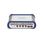

The PicoScope 6000E Series: Capture, control and stream with confidence
Take advantage of best-in-class bandwidth, sampling rate and memory depth.

Power, portability and performance
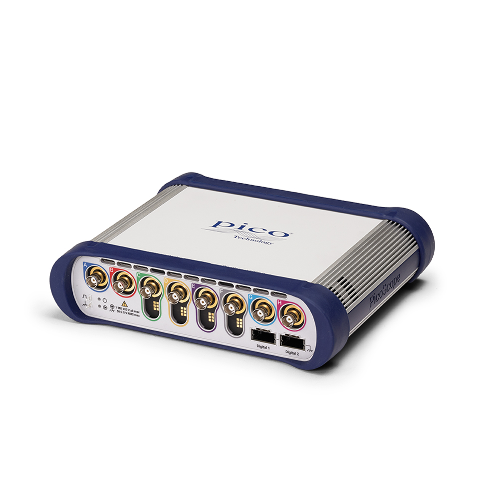
The PicoScope 6000E Series oscilloscopes are as powerful as any traditional scope, with the advantage of a small form that fits easily on your desk. The 6000E Series has oscilloscopes with up to 3 GHz bandwidth, FlexRes® models with up to 12-bit resolution (up to 16-bit with resolution enhancement enabled), plus up to 4 GS of memory – the deepest as standard in its class. With up to eight analog channels plus 16 digital channels and an arbitrary waveform generator able to produce up to 50 MHz signals, to the PicoScope 6000E Series can ably rise to any task.
The ultra-deep memory, combined with 40 serial decoders included as standard, creates an oscilloscope that excels at debugging and monitoring digital systems. At the same time, the careful analog design creates a front end with 60 dB of SFDR, excellent pulse response and minimal crosstalk.
All of these features are accessible through the free PicoScope software, with regular updates, lifelong technical support and no hidden costs.
Flexibility without compromise
The PicoScope 6000E Series works with PicoScope 7, PicoSDK® or PicoLog 6. Combine masks, advanced digital triggers, automated measurements and actions with up to 40 000 waveforms stored in the buffer to spot rare timing errors, glitches and dropouts during long tests with no coding required. Or, use the PicoSDK to create your own applications from scratch.
Unlike old-fashioned SCPI interfaces, our C-based DLLs gives access to every single part of the hardware and can stream up to 312 million samples per second. Integrate a PicoScope 6000E Series oscilloscope into your setup and use the advanced triggers and precise (single sample resolution) trigger timestamping to monitor system performance with no false positives or negatives.
The PicoScope 6000E’s ultra-deep memory is managed on-device with features such as downsampling and data aggregation to reduce latency, while retaining the original capture data if more detailed analysis is required.
Scopes for all needs

Fully-featured oscilloscope…
The PicoScope 6000E Series contains a wide range of oscilloscopes to meet every need. The range starts with excellent value 8-bit, 300 MHz oscilloscopes with 1 or 2 GS deep memory, and extends to 10/12-bit FlexRes® oscilloscopes with up to 1 GHz bandwidth and 4 GS ultra-deep memory, with eight channel models available up to 500 MHz. All of the 6000E Series scopes up to 1 GHz have input ranges from 10 mV to 20 V, AC/DC coupling and 50 Ω/1 MΩ impedances.

… or maximize speed
The PicoScope 6428E-D is an even higher speed version of the standard PicoScope 6000E Series. By limiting the input impedance to 50 Ω only, and reducing the available input voltage ranges, the cost of a 3 GHz oscilloscope has been kept right down. The PicoScope 6428E-D allows you to only pay for what you need and it is ideal for incorporating into OEM applications.
Exceptional mixed-signal performance
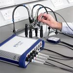
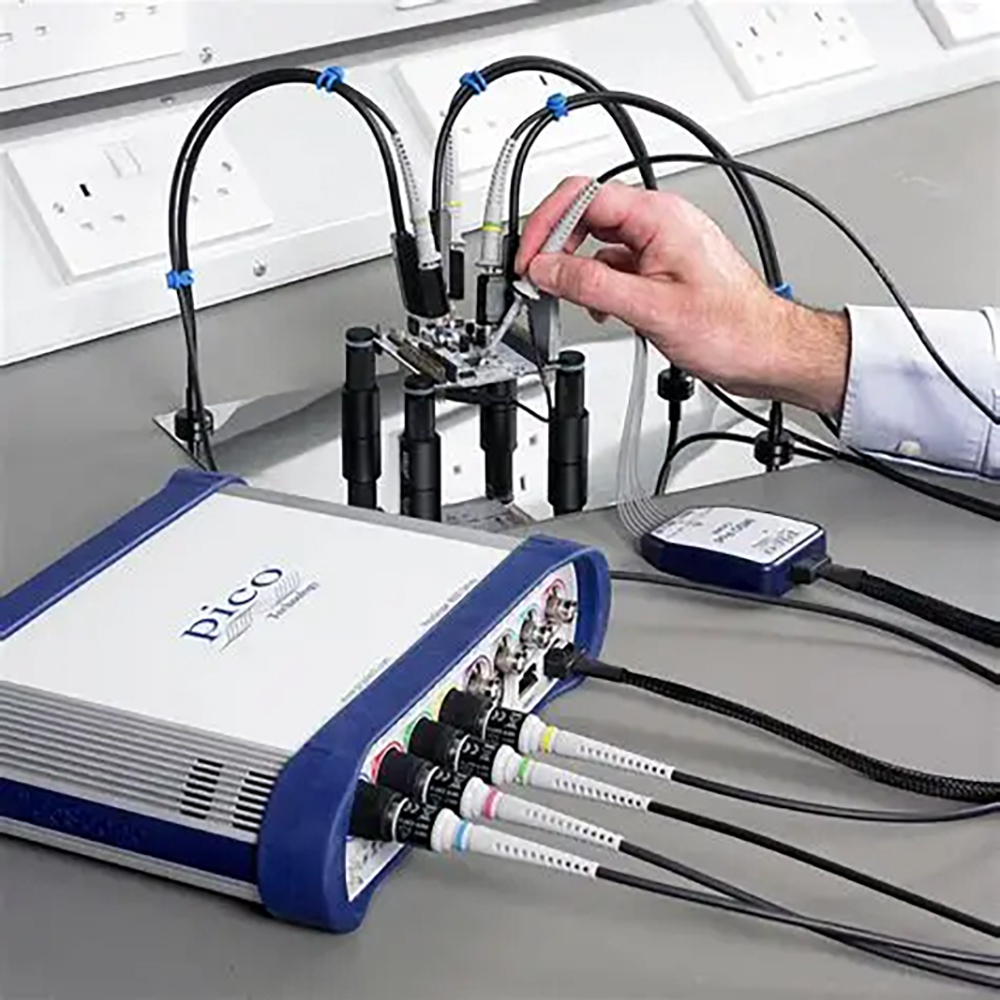
All PicoScope 6000E Series oscilloscopes have two digital ports for connecting to TA369 MSO pods. These pods each have eight digital inputs capable of 5 GS/s operation and a bandwidth of 1 Gb/s (equivalent to a minimum detectable pulse width of just 1 ns). The compact flying leads easily connect to 0.1″ pitch connectors, with minimal loading of the DUT – the input capacitance is just 3.5 pF thanks to high-quality mini-coax flying leads. The external MSO pods give flexibility in probe positioning without compromising on performance or robustness.
Digital channels can be captured at the same time as analog channels so they can be accurately time-correlated and displayed together on screen. Combining digital and analog channels can give you up to 24 channels of data at once – perfect for simultaneous decoding of multiple serial or parallel protocols. PicoScope includes 40+ serial decoders as standard, with new protocols being added all the time as part of the free PicoScope 7 software updates.

The digital channels can be grouped and displayed as a bus on screen (with values displayed in binary, hex, decimal or signed decimal). Alternatively they can be displayed, combined, as a single level – perfect for DAC testing.
Digital channels, like analog channels, work with the wide range of advanced triggers available in PicoScope 7. Digital triggers allow you to define a set combination of levels and transitions so you can capture exactly the condition you need without any false positives. When combined with the 6000E’s deep memory, you can see exactly what conditions led to a certain state.

Ultra-deep memory

PicoScope 6000E Series oscilloscopes can capture up to four gigasamples in their ultra-deep capture memory – many times more than competing scopes. The benefit of deep memory is being able to capture long-duration waveforms at maximum sampling speed. The PicoScope 6000E Series oscilloscopes can capture with 200 ps resolution for 200 ms. For comparison, a scope with a ten megasample memory would only be able to capture with 10 ns resolution for the same time period – that’s 1/50th of the resolution!
An ultra-deep memory is invaluable if you are capturing fast but intermittent signals such as fast serial data with long gaps between packets, or nanosecond laser pulses with millisecond gaps between them. The deep memory can be used to store analog or digital samples, and the capture memory is shared between any channels and MSO ports you have enabled. You can also manually split the memory into up to 40 000 segments. Set up a trigger and store a separate capture in each segment (with as little as 300 ns dead time between captures). Once you have acquired the data you can step through the memory, one segment at a time, until you find the event you are looking for. Each trigger is timestamped with picosecond resolution so you can see exactly when each event occured.
It would be time-consuming to manually search 40 000 segments, so the PicoScope software also includes powerful tools to help you manage your data. Mask limit testing and colour persistence mode can find glitches quickly. The zoom function allows you to zoom into your waveform up to 100 million times, with a Zoom Overview window to easily control the size and location of your zoomed area. Combining the waveform buffer, serial decoders and hardware acceleration with the ultra-deep memory makes the PicoScope 6000E Series some of the most powerful oscilloscopes on the market.
PicoScope 7 – the best keeps getting better

Discover why PicoScope 7 PC oscilloscope software outshines traditional benchtop oscilloscopes and why it’s the choice for professionals seeking performance, efficiency and value.
Comprehensive features at no extra cost: PicoScope 7 includes all essential features as standard, eliminating the need for costly upgrades. Unlike benchtop oscilloscopes that charge extra for options like serial decoders, PicoScope 7 offers 40 decoders included right from the start. Often, it’s more cost-effective to purchase a new PicoScope than to buy just a single serial protocol upgrade for an old benchtop.
Superior display and processing power: leverage the power of your existing computer’s high-resolution display to view up to 10x more detail than a typical benchtop scope. The advanced processing capabilities of your PC allow PicoScope 7 to deliver sophisticated mathematics, measurement, and analysis tools that surpass the capabilities of traditional oscilloscopes.
Seamless connectivity and data management: connecting PicoScope to your PC simplifies saving, sharing, and manipulating data. Effortlessly integrate results into reports, work offline, and share data with colleagues—even those without a PicoScope. This convenience streamlines your workflow and enhances collaboration.
Intuitive and customizable user interface: PicoScope 7 features a user-friendly interface that works seamlessly with both mouse and touchscreen inputs. Available on Windows, Mac, and Linux, you can personalize your workspace by naming channels, choosing color schemes and themes, defining custom probes, pinning frequently used tools for quick access, and selecting from 27 languages.
Future-proof investment: with over 30 years of providing free software updates and feature enhancements, PicoScope ensures your investment remains valuable. Buy the hardware once, and enjoy continuous improvements and new features year after year.
Choose PicoScope 7 for a comprehensive, powerful, and future-proof oscilloscope solution that enhances your productivity and ensures you stay ahead of the curve. More information on PicoScope 7
Smarter serial decoding
Decode more
The serial decoder feature in PicoScope 7 includes a host of tools to make diagnosing and debugging fast and simple. Connect up the MSO cables, assign them to signals and it’s ready to go. PicoScope 7 automatically detects whole frames and divides them up into packets, decoding each one depending on the standard being used. The on-graph display can be configured to show the results in hex, binary, decimal or ASCII so you can line it up with other events.
Choose from a huge selection of protocols, from 10BASE-T1S Ethernet to three- or four-wire SPI to PMBus. Serial decoders can use a mix of digital and analog channels, so with the PicoScope 6804E/6824E that means up to 24 channels of serial data at once. Those channels can decode almost any combination of serial protocols at the same time – the only limit is the bandwidth.

Analyse faster
The PicoScope 6000E Series’ deep memory allows recording of huge amounts of serial data, even across multiple channels. To make analysis of all that information easier, import a link file to translate data from raw numbers to human-readable text, customized to your application. Filter rows and columns to quickly sort and find packets of interest, with errors automatically highlighted.
Statistics give deeper insights into the physical layer such as variation in logic high and low voltage levels. Timing analysis tools help you check the performance of every part of your design and find potential hazards early. Then, easily export recorded data for sharing and publishing.

Waveform buffer and navigator
The ultra-deep memory of the PicoScope 6000E Series oscilloscopes means you can save up to 40 000 waveforms and up to four million samples but there is the risk of that much data being overwhelming. That’s why PicoScope 7 ties together the waveform buffer and navigator with other powerful tools such as masks, measurements and DeepMeasure to produce an extraordinary hardware debugging machine.
Every waveform is stamped with the time it was captured with one-second resolution, plus trigger timestamps – since the first trigger, and since the previous trigger – in one-sample resolution (just 200 ps at 5 GS/s). With this information you can easily cross-correlate different events. Then, use masks and measurements to filter and hide events you don’t need. With the DeepMeasure tool, choose between calculating over the entire memory or just the current buffer, then use the results table to instantly scroll to the time of interest.

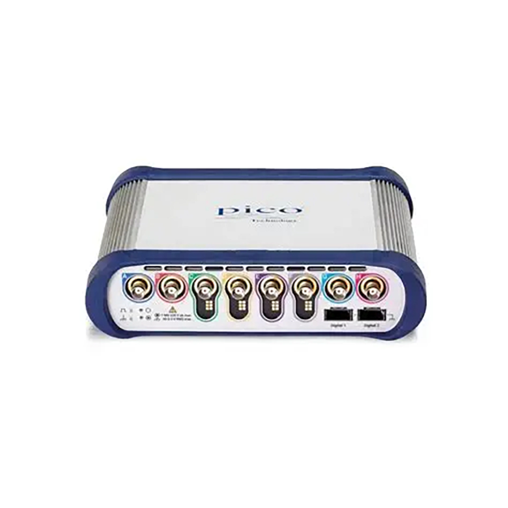
• Four or eight analog channels, with probe detect rings
• Four channels with Pico Intelligent Probe Interface
• Two digital ports for connecting to TA369 MSO pods, for up to 16 digital channels
• Indicator LEDs for power and status
• Probe compensation pins

Spectrum analyser

The integrated FFT spectrum analyzer provides detailed frequency domain analysis, ideal for identifying noise, crosstalk and signal distortion. The spectrum analyzer in PicoScope is of the Fast Fourier Transform (FFT) type which, unlike a traditional swept spectrum analyzer, can display the spectrum of a single, non-repeating waveform. With up to a million points and comprehensive measurement tools, PicoScope’s spectrum analysis capabilities are second to none.
With a click of a button, you can display a spectrum plot of the active channels, with a maximum frequency up to the bandwidth of your scope. To focus on a specific frequency range you can directly set the start and stop values of the analyzer frequency axis.
You can display multiple spectrum views alongside oscilloscope views of the same data. A comprehensive set of automatic frequency-domain measurements can be added to the display, including THD, THD+N, SNR, SINAD and IMD. You can even use the AWG and spectrum mode together to perform swept scalar network analysis.

The spectrum works with the waveform buffer so you can capture and rewind through thousands of spectrum plots. Or, save time by using mask limit tests to scan through them all automatically. Spectrum masks and measurements also work with PicoScope actions just like in the time domain, so you can leave the spectrum running continuously and choose to save the waveform on a mask failure, or trigger an alarm when the harmonics are too high.
A full range of settings gives you control over the number of spectrum bands (FFT bins), scaling (including log/log) and display modes (instantaneous, average, or peak-hold). A selection of window functions allows you to optimize for selectivity, accuracy or dynamic range.
Scopes for a digital world
The world is getting more digital. While analog measurements remain vital in a digital environment (for tests such as signal integrity, rise time, noise and so on), often the data itself within the signal is what matters.
MSOs (Mixed Signal Oscilloscopes) are oscilloscopes with dedicated digital channels as well as the standard analog inputs. These digital channels have just one bit (logic high or low) but instead can measure many channels at once – instead of needing a four channel oscilloscope just to view one bus, an eight-channel digital input can monitor data in, data out, clocks and multiple address lines.

The digital inputs can use any of up to 40 serial decoders (with more being added all the time) as standard, and can even decode multiple different serial protocols at once.
Digital channels can also be displayed as groups with the combined total displayed in a variety of number formats or a single analog value. Advanced logic triggers will wait for a user-defined combination of levels and transitions, so you can customize it completely to your scenario.

Arbitrary Waveform Generator and Function Generator
All PicoScope 6000E Series oscilloscopes come with a built-in function generator and arbitrary waveform generator (AWG) capable of ±5 V output.
The AWG operates at 14 bits and 200 MS/s. By using a variable sample clock, the jitter that typically appears on waveform edges is avoided. In addition, the AWG is capable of generating accurate frequencies down to 100 µHz. AWG waveforms can be created or modified with the built-in editor, imported from oscilloscope traces or loaded from a spreadsheet, and they can be exported to a .CSV file too.
The function generator is capable of sine and square waves up to 50 MHz. It can also create triangle waves, DC voltages, white noise, PRBS and other waveforms at lower frequencies. It includes controls to adjust the amplitude, offset and frequency, plus frequency sweep functions – ideal for testing and validating amplifiers and filters.
Combine the function generator with trigger tools to output a known number of cycles when certain conditions are met, such as the scope triggering or a mask test limit failing.

Flexible resolution, up to 12 bits
What is FlexRes?
A FlexRes® oscilloscope is able to swap between different vertical resolutions, so you can prioritize sampling rate or high resolution, or balance the two. PicoScope 6000E Series FlexRes oscilloscopes make this optimization in the hardware, and so it is more flexible than resolution enhancement or waveform averaging, which are software features. However, FlexRes can be used in combination with resolution enhancement and waveform averaging for even better performance.
An 8-bit scope will have the fastest sample rate and can store more waveforms in its on-board memory. In 8-bit mode your scope can capture and store huge amounts of data for analysis – perfect for decoding digital signals.
A 12-bit scope has 4096 different possible voltage levels, compared to just 256 with 8-bit resolution. The quantization noise of 8-bit mode is much higher, making the SNR much smaller. Using a high vertical resolution is perfect for low-level analog signals when any amount of noise is significant.

How do we do it?
Typically, digital oscilloscopes increase sample rate by time-interleaving multiple low-resolution ADCs. The interleaving process adds fundamental errors so that the dynamic performance is always worse than that of the individual (8-bit) ADC.
Pico’s FlexRes architecture starts with high resolution ADCs, each with multiple cores. The image shows one ADC of a FlexRes PicoScope 6000E Series; with four channels active, each ADC core samples at its maximum rate of 1.25 GS/s. For a single channel, the four cores can be fed with phase-shifted timing signals. Interleaving four high-resolution cores reduces the dynamic performance vs. one single core, but it is still better than a single low-resolution core (but with all the sampling speed benefits).
Alternatively, to prioritise precision over speed, all four cores are fed the same timing signal. The output of the four is averaged to reduce noise and the resolution is boosted to 12 bits. The parallelization improves SNR and non-linearity for excellent dynamic performance.

Ultra-deep memory oscilloscopes
Pico oscilloscopes punch far above their weight in memory depth. Deep memory allows you to capture data for longer, but then zoom in and analyze the data with no loss of horizontal resolution. The zoom function lets you zoom into your waveform up to 100 million times! PicoScope 7 also allows multiple viewports to display the same signal at different zoom levels – see the details without losing sight of the bigger picture.
Ultra-deep memory combines perfectly with measurements and DeepMeasure™ so that you can analyze a huge amount of data at once, for the most accurate statistics. When viewing digital data, the deep memory allows you to record and decode longer periods of communication for more in-depth analysis.

The total memory is divided between all of the active channels, including digital channels if available. The memory can also be segmented in time, so you can set up a trigger and capture data only when it matters – skipping all the dead time in between. Using the PicoScope 7 software, you can have up to a huge 40 000 segments! Searching through that many captures would be incredibly time consuming, which is why the deep memory combines with the waveform buffer, masks, measurements and persistence modes to help you find glitches and errors quickly.
You can also make use of rapid triggering mode, where data is not returned to the PC until all of the segments are full. Pausing communications hugely decreases the re-arm time – perfect for capturing packets of digital data in quick succession. All of the data is stored on the oscilloscope, ready to be retrieved at the end of the capture.

Advanced digital triggers for maximum flexibility

Pico Technology pioneered the use of digital triggers back in 1991 and they have only got more powerful since. The flexibility offered by digital triggers allows for a multitude of advanced digital trigger types – more than just edges, PicoScopes can trigger on runt pulses, different length pulses, or even logical combinations of multiple digital or analog signals. Every trigger is accurately timestamped for reference, displayed as either sample intervals or raw time.
PicoScope uses the actual digitized data to trigger. Time and amplitude errors are minimized through filtering and our digital triggers can trigger on even the smallest signals – there are no limits on slew rate. The trigger is just as accurate at full bandwidth. The trigger levels and hysteresis can be set with the highest precision and resolution.
Digital triggers really excel when it comes to advanced trigger types. PicoScope allows triggers based on signal edges (rising, falling or both) but also pulse characteristics (height, width), timing (rise/fall times, dropouts) and logic. The trigger setup can be a simple threshold, or complex windows so the scope only triggers on what you were actually wanting to see.
PicoScopes with MSOs can trigger when any or all of the 16 digital inputs match a user-defined pattern. You can specify a condition for each channel individually, or set up a pattern for all the channels together using a hex or binary value.
Logic triggers allows you to combine edges and windows on the analog inputs: for instance, trigger on the rising edge of A only if B is already high, or trigger if any channel exceeds a predefined voltage range.
Powerful trigger features
Configurable trigger hold-off
Trigger holdoff allows the oscilloscope to ignore potentially trigger-firing events for a set period of time after a trigger – perfect for finding the first edge of a burst of data but not triggering on the rest, resulting in a clean capture every time. The hold-off can be configured for any period from 1 ns to more than a day!
High-resolution trigger timestamps
Triggers can also be timestamped with single-sample-interval accuracy. With a 10 GS/s sampling rate, that amounts to 100 ps of resolution. With trigger timestamps you can identify precisely when an event took place and easily correlate it with other conditions.

Signal fidelity
PicoScope 6000E Series oscilloscopes have an SFDR of up to 60 dB on FlexRes models. Even on the 3 GHz 6428E-D the crosstalk is better than 200:1 across the entire bandwidth (and over 1000:1 up to 500 MHz). With PicoScope, you can trust in the waveform you see on the screen.

Pico has been designing oscilloscopes for over 30 years. With our experience we design our front-ends to minimize noise, crosstalk and harmonic distortion without compromising on metrics such as pulse response and bandwidth flatness.

Custom probes in PicoScope 7
Custom probes let you correct for non-ideal characteristics in probes, sensors and transducers
Improve readability
Don’t make things more complicated than they need to be: adjust the scaling and units so that you don’t have to keep translating values in your head. With a custom probe you can see the right data at a glance.
Flexible setup
Custom probes can be used to setup a channel with just one click. Configure the coupling, voltage range and filtering to match your hardware.
Advanced lookup tables
Correct for non-linear inputs with a custom lookup table. For example, a non-linear temperature probe can be effectively calibrated so that the correct temperature is displayed on screen and converted to degrees, all in one go.
Configure once, use forever
All your custom probes are saved for reuse and can be saved as part of a .psdata file, so your settings can be shared.


Capture modes
PicoScopes can be configured in many ways so you can gather the data just how you need.
- Block capture
- Rapid trigger
- Streaming mode
In block capture mode, the PicoScope stores captured data in the internal buffer memory, before processing it and transferring it over USB. Once the data is transferred, the next block can begin capturing. The buffer memory is shared equally between each enabled channel.
Block capture mode unlocks the maximum real-time sample rates of your oscilloscope. In this mode, memory communications are half-duplex: the system is only ever reading or writing, never both.

Hardware Acceleration Layer v4
Ultra-deep memory with no lag
With up to 4 GS of memory, 6000E Series oscilloscopes need some clever tricks to keep your computer running smoothly: enter HAL4, our fourth-generation hardware acceleration engine.
The massively parallel design accurately reproduces the signal on the screen while eliminating any bottlenecks from the USB. Your screen update rate stays fast and the controls remain responsive even when storing billions of samples.
Rest assured, though; every capture has been stored on your oscilloscope and can be recalled perfectly at a moment’s notice.
Read more about Pic

Wide selection of probes
Passive high impedance probes
If required, your oscilloscope can be bundled with up to eight passive probes, matched to the bandwidth of your oscilloscope. These high quality probes include a probe detect pin so that your oscilloscope will automatically enable and configure the channel when the probe is connected. The small 2.5 mm diameter makes it easy to see what you are probing.
Active high impedance probes
For minimal-impact probing, connect an A3000 Series probe to the 6000E’s Intelligent Probe Interface. With up to 1.3 GHz bandwidth and an input capacitance of just 0.9 pF, these probes present 50 Ω to the oscilloscope for maximum system bandwidth.
Passive low impedance probes
The TA062 passive 50 Ω probe has 1.5 GHz bandwidth and is ideal for simple probing of high frequency circuits. The probe comes bundled with a variety of adaptors so you can probe ICs without the risk of shorts, as well as ground blade and ground spring accessories for minimizing inductance.
Cross-compatible
All of the PicoScope 6000E Series oscilloscopes are compatible with any standard passive BNC probe – our oscilloscopes have excellent input characteristics without the use of proprietary connectors.


At Pico, we pride ourselves on making high-quality equipment that you can trust, for years to come. That’s why we offer an industry-leading five-year warranty on all our real-time oscilloscopes.

We also offer free support for the lifetime of all our products. Get individual help from our support team of engineers on the phone, by email or on our forum, no matter what you’re working on.

Unlike many other scope manufacturers, we don’t charge to unlock extras on your kit. Everything – all the hardware and software features, plus regular software updates – is included in the price.